Activity 5. Shape from Texture Using Spectral Moments

I. Introduction
A solution to compute the shape of curved surfaces from texture information is presented in the paper of Super and Bovik et.al. In their research work, the authors discussed an accurate method for computing the local spatial-frequency moments of a textured image through the use of Gabor functions and their derivatives. The key in this method is to recover the 3D reconstruction through the tilt and slant of the texture image.

II. Methods
In this activity we were tasked to capture a textured 3D object and reconstruct it by utilizing the Gabor functions and the method used by Super and Bovik et.al. in their research. Another way to find an object with repeating patterns, any object may be wrapped by a repeating pattern like net that is readily available.

The figures below are the ones that I used. With the repeating patterns on the object's surface, the object was reconstructed as mentioned above.

Figure 1. The 3D objects for the reconstruction.

III. Results
This activity is very hard for me. This is done by the researchers for quite some time and me as an amateur to Matlab and image processing know certainly that I cannot do this by myself. That's why I'd like to thank my pretty Loren Tusara for helping me a lot in this activity. Thank you.

So here is the result that I got using the pictures above. These are arranged corresponding to the images in Figure 1.


I give myself a grade of 10. :) Thanks to Loren. Ang hirap ng thesis mo friend.

Activity 7. Stereometry

I. Introduction

There are many ways to render the structure and to measure volumes of different 3D objects. One of the commonly utilized way is stereometry.


Stereometry uses two identical cameras, whose lens' centers are separated by some distance b (see Figure 1). The idea is to combine multiple 2D views to get information on the depth of several points on an object, thereby rendering the 3D object. The plane connecting the centers of our lenses is located at a distance z from the object's location, which is what we want to recover. From the point of view of our cameras one and two, this point appears to be located at a transverse distance x1 and x2 with respect to the centers of cameras one and 2. f here indicates the distance of our image plane from the lenses of the camera. This principle is similar to the principle used by our eyes to perceive depths of objects.

Figure 1. Geometry of the setup used.

In our activity, the setup is simplified further. Since we are using only one camera, we just need to displace the camera to a finite transverse distance, where the lens centers of the two cameras are supposed to be placed when using two cameras. From the geometry in Figure 1, we can derive z as follows:
Applying the camera calibration that we have studied in our previous activity, we can reconstruct the 3D structure that we used.


II. Data Gathering

The raw images used are shown below. This is taken from the group of Kaye from their Applied Physics class.


III. 3D Reconstruction

The following is my reconstructed image using Matlab. From a 2D image, it's still not that good.. I'm having problem with the calibration part of the camera used here since I have to calibrate it again before 3D reconstruction.

I give a grade of 7 to myself here since it's still not good. There was an error in the calibration.

Activity 6. Camera Calibration

--------------------------------------------------------------------------------------
Hayy.. after a very long time of staying as a draft... here is my blog report for the 6th activity. whew!

Introduction
When taking a picture, one can think that the object's world (actual) coordinates are being mapped into the camera's coordinates.

This activity allows us to get the camera properties so that we can get the actual or world-coordinates just from the pictures collected by this camera.

A readily available Matlab Toolbox can be used or one can program his own codes.



Methodology
Pictures of a tsai grid at different orientations are collected. Then the program should successfully trace the squares in the grid. Finally, the program will compute for the camera properties using two methods:

A. Camera calibration using the available Matlab toolbox from the internet, and
B. Camera calibration using our own codes. In this part, two Tsai grids are oriented perpendicular to each other.

Shown in Figure 1 are five of the 17 images I used for part A, and shown in Figure 2 is the Tsai grid I used for part B.

Figure 1. Few of the figures I used for part A of this activity.

Figure 2. The image used for calibrating the camera using own code.

Results
A. Figure 3 shows the calibration done for images in Figure 1. As one can see the corners of each of the squares are correctly predicted. As a plus from the toolbox, the errors and the extrinsic parameters can also be computed. Here i computed it and the results are shown in Figure 4.

Figure 3. Camera calibration results using the available toolbox.


Figure 4. The computed errors and the extrinsic parameters of the camera.

B. For part B, I had a hard time since I had to click all the input points for the program. I had to click at least 25 points and one mistake... just one mistake... will bring me back to zero. So for this part, Rene kindly offered his help not only in the Matlab program but also in clicking the images when I got too upset repeating the clicking process for the 3rd time.

Figure 5s is a sample of my failures in clicking the Tsai grid. hehe :) And Figure 5b shows the correct calibration done.


I put in a lot of effort in this activity especially patience. :) I give myself a grade of 9 for I posted my report so late. :)

Activity 1. Adaptive Segmentation and Tracking Using the Color Locus

Introduction

In this activity, an adaptive histogram backprojection method is utilized to track the face of the subject in a video clip, under varying illumination. This is done by creating a color locus first.

The color locus is estimated using the rg-histograms of selected pre-cropped pictures of the subject's skin under varrying illumination. The video is then parsed into image frames, where a frame-by-frame histogram backprojection is done. This histogram is adapted based on the object locus.

Before doing this, I reviewed the concept of histogram back-projection using Scilab (I hope to put up my blog for this topic later). Then I used VirtualDub for parsing the video of Kirby and then I moved to Matlab for the rest of this activity.


Results
The processing of the subject's video is now done using Matlab. A successful implemetation as seen below is an unbroken tracking of the subject's face under varying illumination.

Figure 1. Tracking the face of the subject.

Successful tracking of the subject's face was obtained even when the subject was under varrying illumination as seen in the above figure.

For this activity, I give myself a grade of 10 for I could track the face of Kirby (the subject ^^) under different illumination and I exerted a lot of effort from reviewing in Scilab to finally implementing it in Matlab.

Thanks to the graduating batch for teaching me especially when I was reviewing histogram backprojection in Scilab. ^^

Reference:
1. Physics 305 handouts by M. Soriano
2. Soriano, Martinkauppi, Huovinen, Laaksonen, Adaptive skin color modeling modeling using the skin locus for selecting training pixels, Pattern Recognition, Vol. 36, No. 3, March 2003

Activity 4. High Dynamic Range Imaging

INTRO(?) ^^
When Ma'am Jing discussed how they applied this HDR to mammogram images, it amazed me. At that same time though, the title of this activity blew me off. It sounded so complicated. A contributing factor was the fact that we're supposed to use it to view plasma(another word that I don't know much), for Kuya Leo's Lab work. As a result, I ignored it. I thought I could get away from this activity. But noohh...

It can't be helped. I have to do it. When I was doing it, I realized the activity was easier than I first thought and imagined.


The goals for this activity are to:
1. solve for the response function g(Z) of a camera using the steps outlined in the paper of Devebec and Malik 97 and
2. render a high dynamic range image of the picture by solving for the irradiance given g(Z), the shutter speed for each image, and pixel value.



METHODS
In attaining the first goal, I just followed the steps in the abovementioned paper, as follows.
1. I took pictures of the plasma in Plasma Physics Laboratory of National Institute of Physics Philippines (thanks for the permission) for varrying shutter speeds. The camera was set so that there must not be any lateral movement when taking the pictures.
2. Next, I picked 5 points for each of the images taken. Note again that each image corresponds to one shutter speed (as these were taken at different speeds).
3. The plot for ln(shutter speed) against gray level values (Z) is obtained. And using the least square method outlined in the abovementioned paper, the g(Z) response function og the camera is obtained.

RESULTS
Shown in the figure are the images that we were able to take from Plasma Lab and the corresponding shutter speeds used for our camera.

Figure 1. The input images used.

Table 1. The corresponding shutter speeds used in capturing the images in Figure 1.

My first plot is the plot of ln(shutter speeds) vs gray-level values(Z), as follows.

Figure 3. Plot of gray values(Z) as a function of Ln(shutter speed).

After getting this plot, a fit is obtained through the method and Matlab code mentioned in the paper of Devebec and Malik 97. In their work, they used the method of least squares. Shown in the following figure is the response function of the camera, g(Z).

Figure 4. The response function of the camera.

The first of the two goals is now obtained. The next step is now to render a high dynamic range image of the picture by solving for the irradiance from the given values. I'm still thinking how to render an image using the irradiance here...

To be continued....

Activity 3. Tracing Silhouettes via Freeman Vector Code

On Silhouettes..

This activity is taken from the paper of A. Araullo, Dr. Soriano and Dr. Saloma on gait-analysis as a possible biometric authentication [1].

-----------------------------------------------------------------

This activity can be summarized into four steps:

1. Capture an object against a plain background
2. Get the edge of the object and its (x,y) coordnates and convert it to a Freeman vector chain code.
3. Take the information on the curvature of the result in 2 by getting the difference between the current and previous pixel and performing a running sum.
4. Finally, the result in 3 is superimposed to the (x,y) coordinates of the edge detected in two showing chains of zeros as region of straight lines, negarics as region of concavities and positives as regions of convexities.

Writing blogs reports for my activities stresses me because of its technicalities that are not of my field (and that are very new to me), so please allow me to make this a little more fun by playing around with the titles. (wink(*-^))
________________________________________________________________________________________
I. Nakatatak sa isang litrato.
For my object, I used a picture of a toy duck that I took from the internet [2].

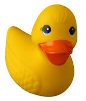
Figure 1. The toy-duck picture used for the activity.

II. I-Follow ang edgy life. (I think physicists live a lives that're always at the edge.)

The edge of the object is extracted using the built-in tool for edge detection in Scilab. I encountered a problem in this early part of the activity for the edges of the eyes of this duck was also detected. I had to detect edges of small size by using find command and merge it with the background.

Then I used follow command to store the (x,y) coordinates of its edge into an array the way it follows the countour. Plotting the coordinates given by the follow command gave me this binary image.

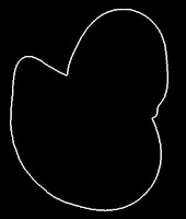
Figure 2. Getting the edge of the duck and following it with follow.

In this part, I encountered another problem again. Since the edge detected in the previous step was not one pixel-thick, the follow command followed too many points. At first I was confident with the output of edge detection in scilab so I didn't think of verifying the output if it's just one-pixel thick. Unfortunately I was wrong. So I had to use thin to reduce this to size of 1 pixel. I found however that the equivalent thin command in Matlab is better (with the help of Kaye commenting on this plot.) So Kaye 'thinned' this plot for me in Matlab because I didn't have my own Matlab at that time (this was the time I was still sticking with memory-efficient (?) Scilab).

Then I had to encode my Freeman vector code. It took me a while (hours and I think days) to think about this Freeman code. The concept is okay but as for me, my creativity was in a vacation (I was too pre-occupied with teaching stuffs and my own research experiments at the lab) that I couldn't even imagine (or I didn't want to imagine) how to program this. Until the time that it dawned on me to finish this activity for I was already getting stuck in this for about about a week since I started it. And so I encoded it.

So here is how the Freeman vector code works. I started with the first element of my array of the edge coordinates. This is in a sense the same with follow command but instead of returning the coordinates, we assigned an integer from [1,8] indicating the direction of the next pixel based on its position measured with respect to the current-pixel location, as shown in Figure 3. For example, the next pixel is to the upper right corner of the current pixel then we label the next pixel with number 3.

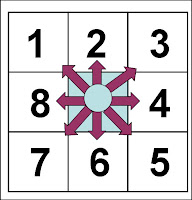
Figure 3. Freeman vector code. The next pixel is labeled [1,8] based
on the orientation with respect to the current pixel position.

III. Geeky mode
With successful conversion to a freeman code, we are now ready to get the difference between two successive pixel values and store it to a new array. Then from this array, we get the running sum of three pixels and put it into a new array, as shown in the figure below.

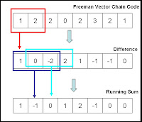
Figure 4. From the Freeman vector chain code, the difference between two consecutive
numbers is calculated. After which, a running sum of three elements is done
resulting to a one-dimesional array of zeroes, positives and negarics.

IV. Eureka!

Finally (whew!). The last part is now to overlay the result in the running sum into the coordinates of the edges calculated earlier with the follow command. At this moment, Scilab has no built-in function to do that so I had to switch to Matlab, else it'll take more time (again!). We expect a plot of the contour of the image used but instead of plot of points, its a plot of numbers where zeroes indicate regions of straight lines, negarics as regions of concavities and positives as regions of convexities. This is easy with the built-in function text(x,y,'a') in Matlab. Here is what I got with the pretty toy-duck picture.

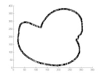
Figure 5. The result of running sum superimposed with the edge coordinates.

Figure 6. Zooming in at the duck's tail in Figure 5.

This is the last goal for this activity, which I achieved after more than two weeks considering the delays it took me to debug my program. For this activity I give myself a grade of 10.

Thanks to those who shared with me some academic noise that served as catalyst of this activity.

References:
1. A. Araullo, M. Soriano, C. Saloma. Curve Spreads - a biometric from front-view gait video. Pattern Recognition Letters 25(2004) 1595-1602.
2. https://www.ftcmain.co.uk/live/pages/images/duck.jpg

Activity 8. Gray-Code Illumination Technique in Rendering 3D Objects

Gray Code Illumination Technique

Gray-code illumination is usually used in rendering 3D shapes and structures. Unlike other methods that render 3D objects, e.g. photometric stereo and stereometry, this method requires only one surface view of the objects. Another good thing about this method is non-invasive.

Methods
The detailed method used in this activity is completely adapted and thus can be seen from the work of K. Vergel and M. Soriano [1] and this method is used with the help of K. Vergel.

Gray-code illumination uses binary patterns that are projected along the Y-axis. In our activity, we used black and white stripes with respective logical values of 0 and 1. n patterns result to 2^n unique code sequence. Patterns with higher stripe frequency result to a more accurate 3D reconstruction.

Figure1. Bit planes and bit-plane stack.

Figure 1 demonstrates how this method works. Three stripe patterns (called bit plane) are projected one at a time, and stacked together (bit plane stack) as shown. For n=3, we have 8 unique code sequence (see Table). Each row corresponds to a pattern while each column corresponds to a single light plane. If a line is drawn (blue line) through the stack of planes, we see that that line has a unique label provided by the logical value of the patterns. This label is the unique code sequence for that plane (column) which enables a one-to-one correspondence betweem the image location and points on the object plane.

Figure 2. The experimental set-up.

Figure 2, shows how the object's dimensions are computed using this method. First, the stripe patterns fromo the projector P are projected unto the Q plane. Lines PU and PK are imaged by the camera C into U'(i, j) and V'(i, j), respectively. The camera will record the images of the stripe patterns without any distortion and this is our 'control' for our activity. After which, the 3D object with height z(x,y) is placed on plane Q. This time, the previous projection of lines PU and PK are now represented by new points G and F. These new points are now projected in the camera as U'(i, j) and V'(i, j*). The shift in the pixel (or line distortion of the patterns) are measured as
From Figure 2, the height of the image can now be computed using the following equation.

In this activity, we tried to render a pyramid using eight stripe patterns. The setup is calibrated by K.Vergel, and the processing is done using the ever useful Matlab.

Results

Figure 3. Stripe patterns on plane Q.

Figure 4. Distorted stripe patterns projected unto a pyramid.

Shown in Figures 3 and 4 are the patterns projected unto plane Q and unto the pyramid object. Figure 5(a,b) shows the reconstructed 3D object viewed from two different angles.

(a)

(b)

For finishing touches, the median filter is used for smoothened surface shown in the figure below.
For this activity, I give 10+ 2 points since I put in a lot of effort and finished it well. (wink*) Kaye, ayos tong thesis mo. :)

Thanks to Irene, and Kaye! The best kau. (ehem... Thirdy, oo na, kaw na pinakamagaling sa kanila sa matlab. hehe)

References:
[1] K. Vergel, M. Soriano. Volume estimation from partial view through gray-code illumination technique. Proceedings of the Samahang Pisika ng Pilipinas, Oct 2008.